Original URL: https://www.theregister.com/2014/05/23/big_data_nyquist_shannon_sampling/
Big data hitting the fan? Nyquist-Shannon TOOL SAMPLE can save you
Lessons from information theorists brainboxes - in pictures
Posted in On-Prem, 23rd May 2014 09:04 GMT
Big Data's Big 5 You are working on a big data project that collects data from sensors that can be polled every 0.1 of a second.
But just because you can doesn’t mean you should, so how do we decide how frequently to poll sensors?
The tempting answer is to collect it all, every last ping. That way, not only is your back covered but you can also guarantee to answer, in the future, all the possible questions that could be asked of that data.
When dealing with transactional data I certainly default to the “collect it all” approach because generally the volume of transactional data is much lower. But with sensor data there can be a real trade-off.
Suppose you can capture all of the data (10 times a second) at a cost of £45m per year. But you could also collect data once every 100 seconds (which is 0.1 per cent of the data) for 0.1 per cent of the cost, a measly £45,000. Are all those tiny little details really worth the extra £44,955m?
More importantly, how do you make the decision?
Welcome to Nyquist–Shannon sampling, also known as Nyquist Theorem, from Harry Theodor Nyquist (1889–1976) and Claude Elwood Shannon (1916–2001).
Nyquist was a gifted student turned Swedish émigré who'd worked at AT&T and Bell Laboratories until 1954 and who earned recognition in for his lifetime's work on thermal noise, data transmission and in telegraph transmission. The chiseled Shannon is considered the founding father of the electronic communications age, who devised the concept of information theory while working at Bell Labs in the 1940s. His award-winning work looked at the conditions that affect transmission and processing of data.
Their theorem has since been used by engineers to reproduce analogue (continuous) signals as (discrete) digital and look at bandwidth.
Let’s think about a real example where their theory might help us: polling smart electricity meters at regular intervals. If the sole analytical requirement is to monitor usage on a daily basis it doesn’t require a genius to work out the required sampling rate. But suppose we are given a broader specification.
Say your client tells you: “We know that our customers have appliances that come on and off on a regular cycle (fridges, freezers etc) and we want to analyse the usage of those individual appliances.”
I can’t tell you how to perform the analysis (I’d need more information) but I can instantly put a lowest limit on how frequently you need to sample in order to be able to guarantee this ability.
Take the appliance that switches on and off most rapidly and sample slightly more than twice as often as it switches. So, if it switches on once every 20 minutes and off about 10 minutes later (so it goes on and off about three times an hour), you should sample just over six times an hour.
As said, our answer is Nyquist–Shannon, which states:
If a function x(t) contains no frequencies higher than B hertz, it is completely determined by giving its ordinates at a series of points spaced 1/(2B) seconds apart.
Adjust your frequency
In practice, for reasons I’ll explain below, although sampling at just over twice the frequency is in theory adequate, you may well want to sample more often than this. But the huge advantage of the Nyquist-Shannon theorem is that it sets an absolute minimum.
This is all much better illustrated by a mix of diagrams and words. Imagine that you want to digitise an analogue signal whose highest frequency component is 1,000Hz. The Nyquist theorem tells us we must sample at a minimum of 2,000 times per second (twice the highest signal frequency).

Let's start by looking at a wave, below.
To illustrate why Nyquist says we need to sample at just over twice the frequency of the signal, let’s try not doing it. In the next illustration I am sampling at just under half the frequency.

My sampling “sees” a wave form of a much, much longer wave length than the original analogue one.

OK, let’s sample more frequently. In the next illustration I am sampling at exactly twice the frequency. If I was really unlucky I would see no signal at all.

If I was really lucky I would see it perfectly, below.

And we could have anything in between, but most of the time I would detect the frequency. Here I am sampling at just over twice the frequency. This detects the frequency, but it is barely adequate (as you can see).

Although I can try to algorithmically predict the original frequency:

In the next illustration, below, I am sampling at around eight times the frequency, which is perfectly adequate – note the scale change.
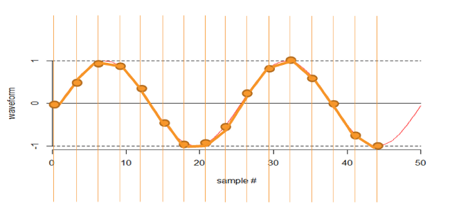
So, that is the basis of the Nyquist–Shannon sampling theorem. Of course, household appliances don’t usually produce sine waves, they usually produce essentially square waves because they are either on or off. So let’s have a look at some (more or less) square waves.
If I sample at far less than the frequency, my sampling “sees” a wave form of a much, much longer wave length, as you can see in the next illustration:

Sampling at just over twice the frequency picks up the wave but loses detail:

Sampling at about eight times the frequency gives you what you need - note the scale change.

So, let’s think about sampling theorem in terms of sampling power usage in a private house. The fridge turns on and off at 20-minute intervals. If you sample at one hour intervals, you essentially cannot see the fridge. If you sample at 10-minute intervals, you can see every cycle of the fridge but, in practice, you will almost certainly want to sample more frequently, perhaps every five minutes.
Nyquist–Shannon developed their theorem during the white heat of computing’s dawn – their ideas were incubated in hothouse for innovation Bell Labs.
Their principles were conceived in the world of telecommunications but are relevant to today's challenges in big data – a world where many follow the herd in hoovering up all they can and worrying about the details later.
With Nyquist–Shannon, you get the insight minus the overload. ®
Enjoyed this? See our earlier Big Five articles here and here, and look out for the final two next week.